LKJ correlation distribution in Stan

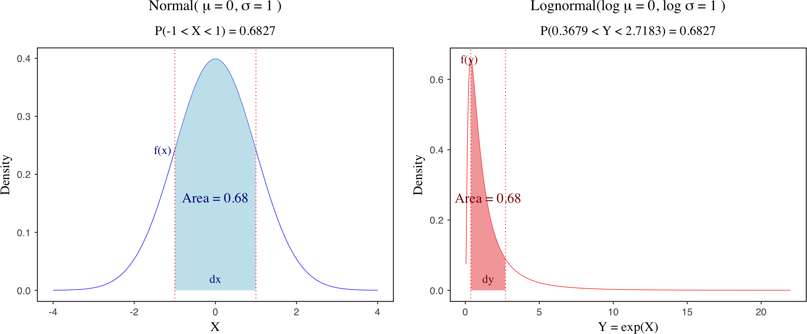
Lewandowski-Kurowicka-Joe (LKJ) distribution is a very useful prior distribution for parameter estimation in correlation matrices, and is also tightly related to matrix factorizations such as Cholesky decomposition. For example, when you use Cholesky decomposition to decompose a variance-covariance matrix ($\Sigma$​) into the multiplication of 3 matrices, you can set $\text{LKJCorr}$​ prior for the correlation matrix $\text{R}$​​.

1. Form

Its probability density function is defined as:

where $c_d$ is the normalizing constant for the dimension $d$​, and can be represented in the following equation (see Lewandowski et al. 2009 for details).

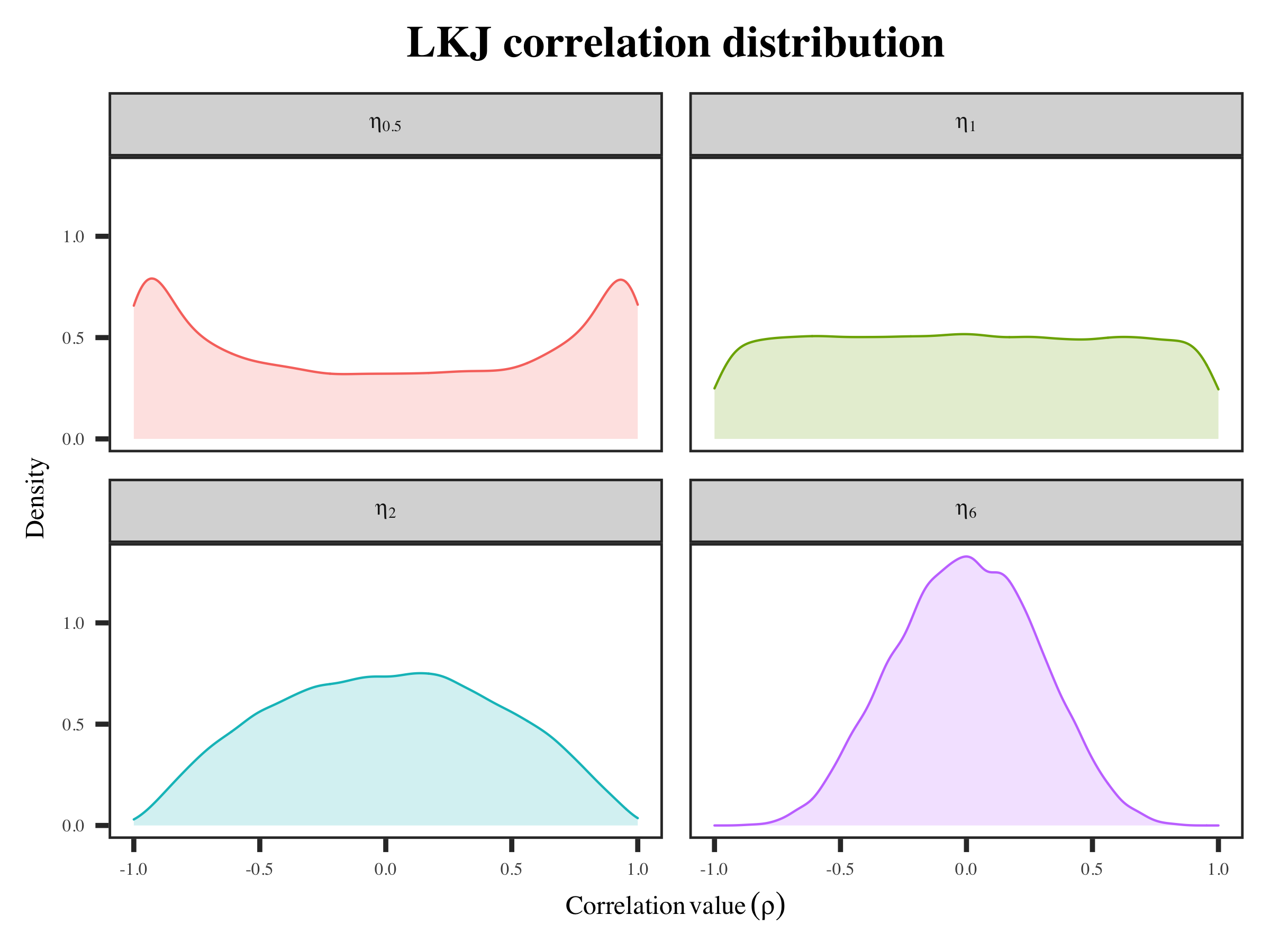
The $\text{LKJCorr}$ prior is used for a positive-definite, symmetric matrix with unit diagonal (i.e., a correlation matrix ($\text{R}$) with main diagonal as 1 and off the diagonal elements as $\rho$). The shape parameter $\eta$ is used to determine the shape of the probability density function. It can be interpreted like the shape parameter of a symmetric beta distribution (see the stan function reference).

• if $\eta = 1$, then the density is uniform over correlation matrices of a given order $K$ (the number of row/column). This suggest we do not know whether there is a correlation or not. The correlation values can be anything between 0 and 1.

• if $\eta > 1$, the correlation values in correlation matrices are going to centered around 0. higher $\eta$ indicate no correlations (converge to identity correlation matrix).

• if $0 < \eta < 1$​​​, the density will centered at two ends. This means correlations are favored, but both positive and negative correlation values are equally possible.

  

2. Data

To make it clear, we can extract the lkj_corr_rng function from stan, and generate some pseudo-data.

my_lkjcorr_fun = "
functions {
  // generate lkj correlation matrix (R)
  matrix my_lkj_corr_rng(int K, real eta) {
    return lkj_corr_rng(K, eta);
  }
  
  // generate cholesky factor L
  matrix my_lkj_corr_chol_rng(int K, real eta){
  return lkj_corr_cholesky_rng(K, eta);
  }
  
  // perform triangular matrix multiplication L*L^T
  matrix my_multiply_lower_tri_self_transpose(matrix L){
    return multiply_lower_tri_self_transpose(L);
  }
}
"
expose_stan_functions(stanc(model_code = my_lkjcorr_fun))

Here we are using the function of expose_stan_functions to export the above stan functions to R. Let’s first generate some matrices via these newly defined functions.

# randomly generate a correlation matrix (R)
my_lkj_corr_rng(K = 2, eta = 1.4)
#           [,1]       [,2]
#[1,]  1.0000000 -0.8743114
#[2,] -0.8743114  1.0000000

# randomly generate a Cholesky factor (L)
(L_chol = my_lkj_corr_chol_rng(K = 2, eta = 1.4))
#           [,1]     [,2]
#[1,] 1.00000000 0.000000
#[2,] 0.09454103 0.995521

# triangular matrix multiplication (L*L^T)
# L_chol %*% t(L_chol)
my_multiply_lower_tri_self_transpose(L_chol)
#           [,1]       [,2]
#[1,] 1.00000000 0.09454103
#[2,] 0.09454103 1.00000000

With these functions, we can generate 100 correlation matrices and try to estimate the parameter $\eta$​​ in the LKJ correlation​ distribution.

# y: a list of 100 matrices
y = map(1:100, ~ my_lkj_corr_rng(K = 2, eta = 1.4))

# data_lkj_corr: a list of list
data_lkj_corr = list(N = 100, y = y)

Note that the array in stan is similar to a list of list in R. If you feed in the data as a R array, the dimension will not match. Also, stan supports mixed indexing of arrays and their vector, row vector or matrix values. For example, if m is of type matrix[,], a two-dimensional array of matrices, then m[1] refers to the first row of the array, which is a one-dimensional array of matrices.

3. Model and Results

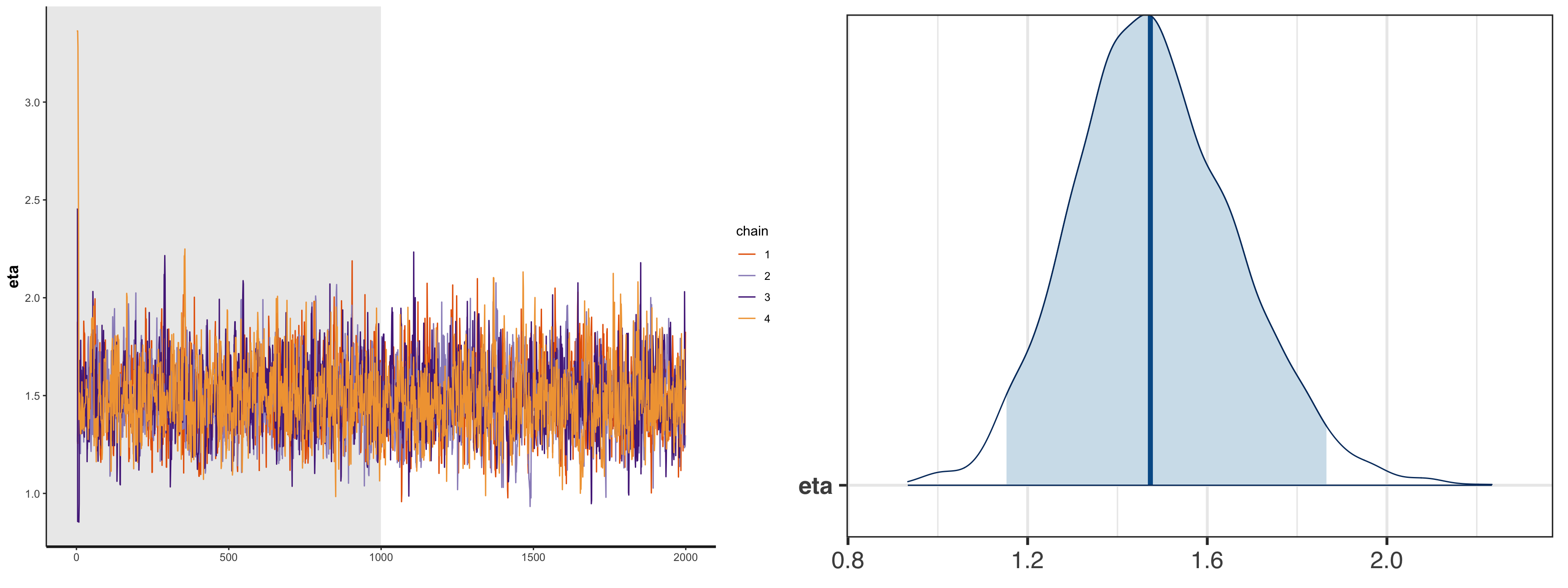
With the simulated data, we can run the following stan model and visualize the posterior distribution of parameter $\eta$.

data{
int N; // number of observations
corr_matrix[2] y[N]; // A n-element arrary of observed correlation matrix [N, 2, 2], equivalent to a list of matrix in R
}
parameters{
real<lower=0> eta; // estimated parameter
}
model{
for(i in 1:N){
  y[i, ,] ~ lkj_corr(eta); // y[i,] and y[i, ,] should also be fine
  }
}

fit_lkj_corr = sampling(stan_lkj_corr, data=data_lkj_corr,
                          chains = 4, iter = 2000, cores = 4)
print(fit_lkj_corr)
#       mean se_mean   sd   2.5%    25%    50%    75%  97.5% n_eff Rhat
#eta    1.48    0.01 0.18   1.15   1.36   1.47   1.60   1.87  1263    1
#lp__ -65.07    0.02 0.73 -67.08 -65.21 -64.78 -64.61 -64.56  1664    1

Useful links:

• https://yingqijing.medium.com/multivariate-normal-distribution-and-cholesky-decomposition-in-stan-d9244b9aa623
• https://mc-stan.org/docs/2_27/functions-reference/lkj-correlation.html
• https://distribution-explorer.github.io/multivariate_continuous/lkj.html
• http://stla.github.io/stlapblog/posts/StanLKJprior.html