Nested or Splitted Structures in Data Simulation and Inference

The development of dplyr and purrr packages makes the workflow of R programming more smooth and flexible. The dplyr package provides an elegant way of manipulating data.frames or tibbles in a column-wise (e.g., select, filter, mutate, arrange, group_by, summarise and case_when) or row-wise (rowwise, c_across, and ungroup) manner. It also fits well with the map function by applying an anonymous function to each column, or applying a user-defined function to each row.

The purrr package allows us to map a function to each element of a list. You can also select, filter, modify, combine and summarise a list (see this blog for an overview). Note that the default output from map function is a list of the same length as the input data, though you can easily reformat the output into a data.frame via map_dfr and map_dfc functions.

Here we focus on comparing and understanding the nest and split functions in data simulation and inference. Specifically, two data structures (nested data vs. splitted data) are used for simulating and fitting linear regression models across different types.

1. Linear regression via nested structures

(1) Function

We first define a function to generate the response (y) by providing the predictor (x), intercept and slope.

# function to generate the response
generate_response <- function(x, intercept, slope) {
  x * slope + intercept + rnorm(length(x), 0, 30)
}

(2) Simulation with given parameters

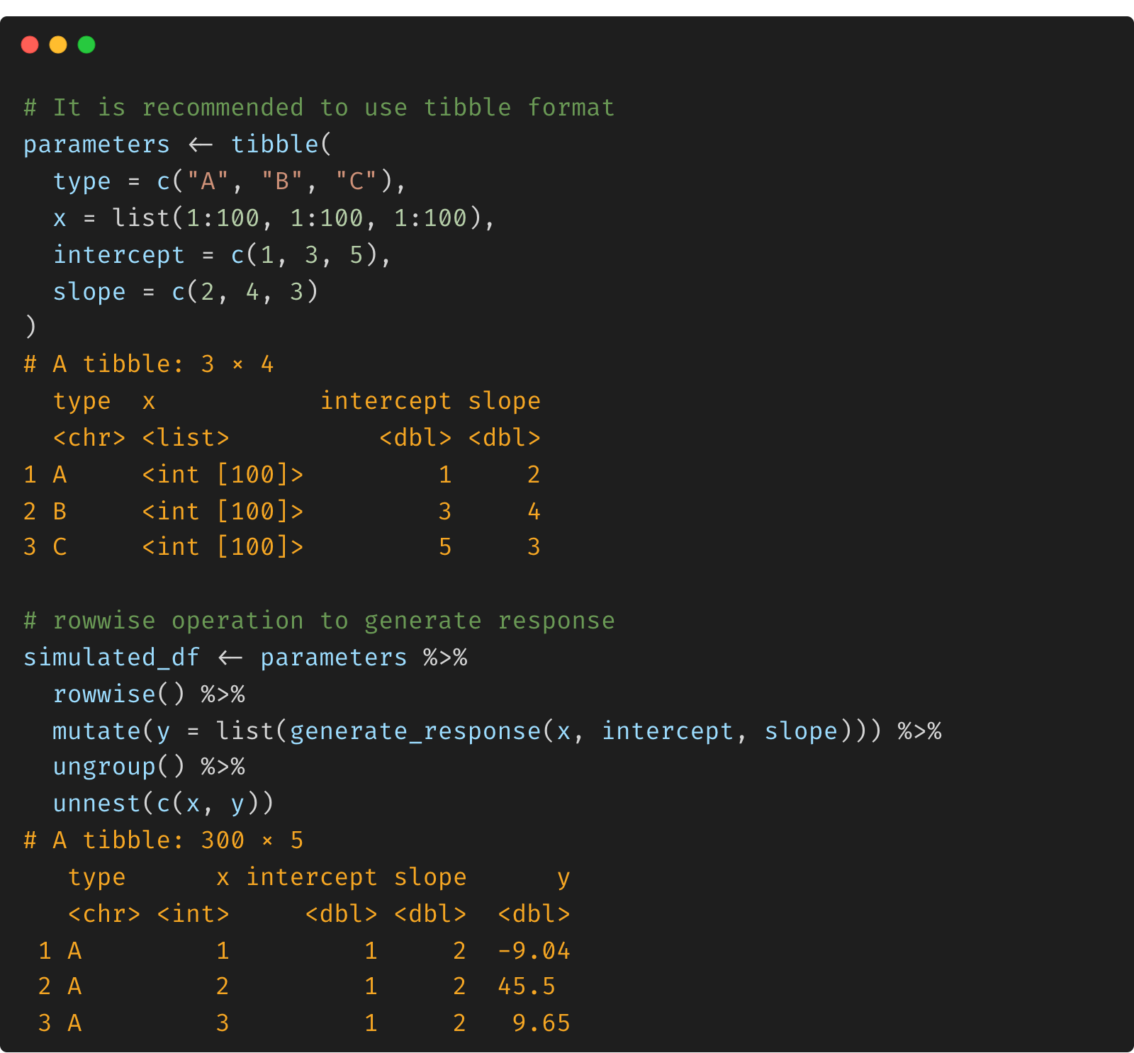
To simulate data for each type (A, B or C), we put the parameters in a tibble, since it allows nested objects with a list of vectors as a column. To generate the response, we use a rowwise function by applying the generate_response function to each row.

# it is recommended to use tibble format
parameters <- tibble(
  type = c("A", "B", "C"),
  x = list(1:100, 1:100, 1:100),
  intercept = c(1, 3, 5),
  slope = c(2, 4, 3)
)
# note: convert the vector responses into a list
simulated_df <- parameters %>%
  rowwise() %>%
  mutate(y = list(generate_response(x, intercept, slope))) %>%
  ungroup() %>%
  unnest(c(x, y))

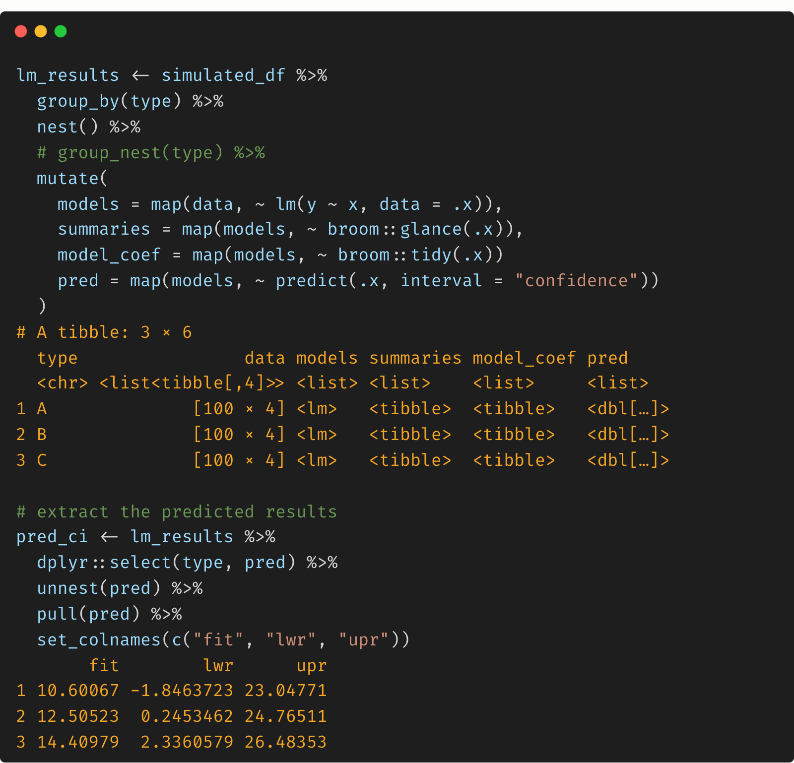
(3) Run the linear model

With the simulated data.frame or tibble, we can create a nested data and map the linear model for each type. After that, we can extract the predicted values and 95% credible intervals.

# nesting data by each type and run lm via map
lm_results <- simulated_df %>%
  group_by(type) %>%
  nest() %>%
  mutate(
    models = map(data, ~ lm(y ~ x, data = .x)),
    summaries = map(models, ~ broom::glance(.x)),
    model_coef = map(models, ~ broom::tidy(.x)),
    pred = map(models, ~ predict(.x, interval = "confidence"))
  )
# extract the predicted results
pred_ci <- lm_results %>%
  dplyr::select(type, pred) %>%
  unnest(pred) %>%
  pull(pred) %>%
  set_colnames(c("fit", "lwr", "upr"))

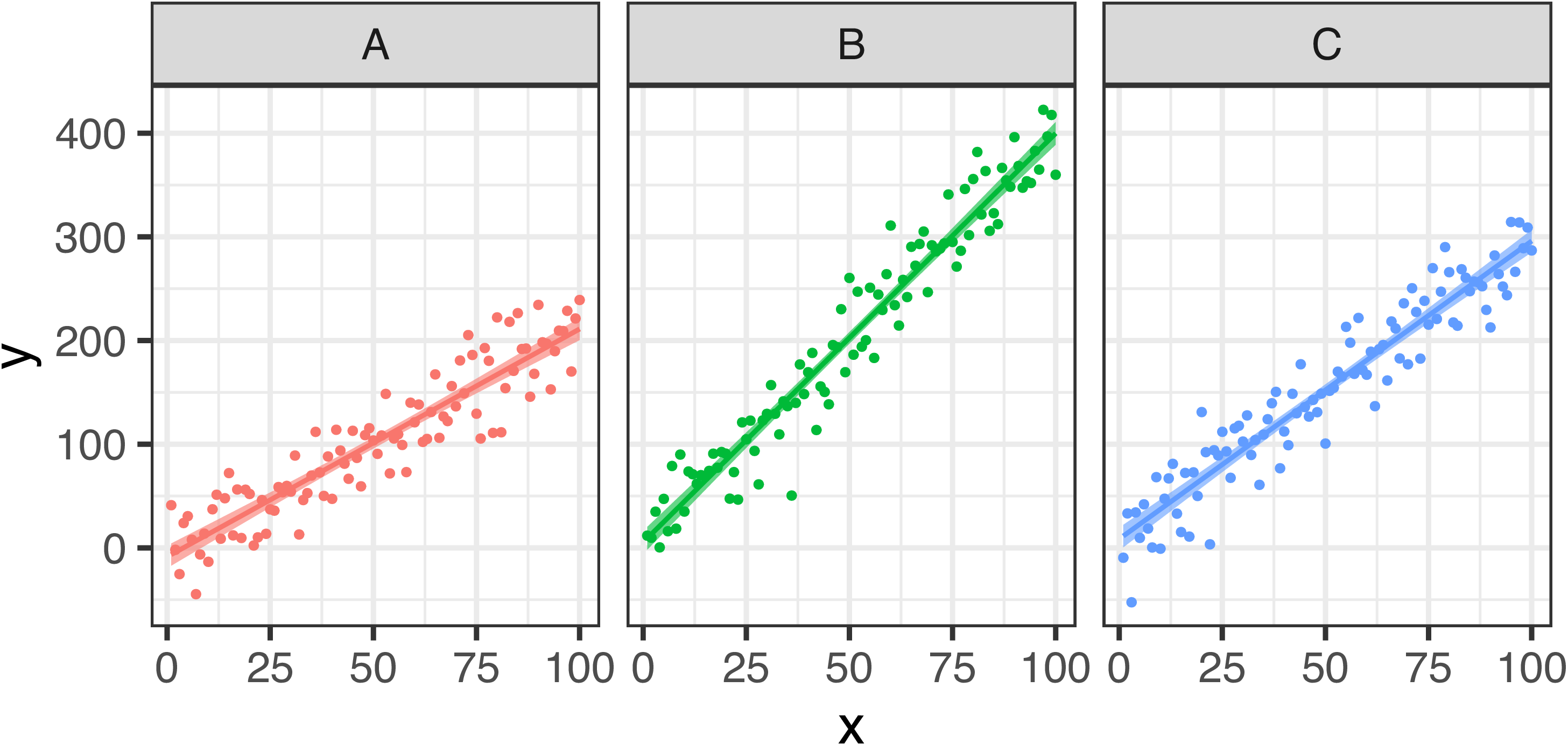
(4) Visualization

To visualize the raw data and the fitted lines, we need to combine them by row, and draw the fitted line and credible intervals via geom_line and geom_ribbon functions from ggplot2.

cbind(simulated_df, pred_ci) %>%
  ggplot(., aes(x = x, y = y, color = type)) +
  geom_point() +
  geom_ribbon(aes(ymin = lwr, ymax = upr, fill = type, color = NULL),
    alpha = .6
  ) +
  geom_line(aes(y = fit), size = 1) +
  facet_wrap(~type) +
  theme(legend.position = "none")

2. Linear regression via splitted structures

Alternatively, we can split the simulated data by each type and replicate the whole analysis by using map functions. Note that you may still need to convert the data into a data.frame so as to combine them by row.

parameters <- list(
  type = c("A", "B", "C"),
  x = list(1:100, 1:100, 1:100),
  intercept = c(1, 3, 5),
  slope = c(2, 4, 3)
)

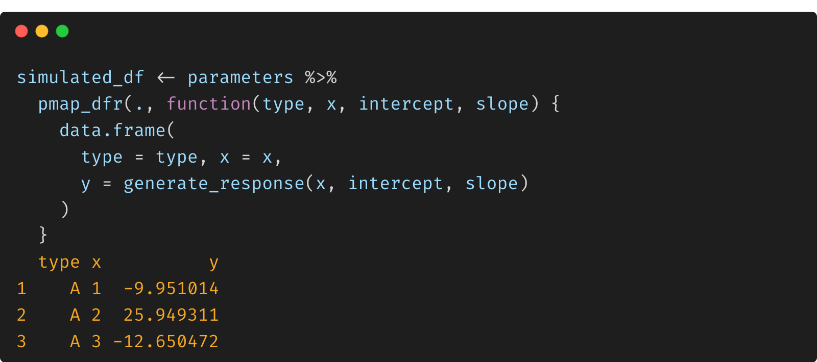
simulated_df <- parameters %>%
  pmap_dfr(., function(type, x, intercept, slope) {
    data.frame(
      type = type, x = x,
      y = generate_response(x, intercept, slope)
    )
  })

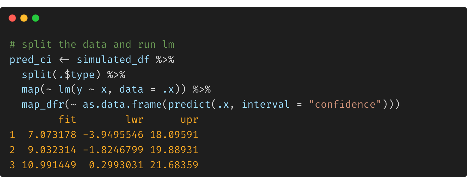
pred_ci <- simulated_df %>%
  split(.$type) %>%
  map(~ lm(y ~ x, data = .x)) %>%
  map_dfr(~ as.data.frame(predict(.x, interval = "confidence")))

cbind(simulated_df, pred_ci) %>%
  ggplot(., aes(x = x, y = y, color = type)) +
  geom_point() +
  geom_ribbon(aes(ymin = lwr, ymax = upr, fill = type, color = NULL),
    alpha = .6
  ) +
  geom_line(aes(y = fit), size = 1) +
  facet_wrap(~type) +
  theme(legend.position = "none")

3. Concluding remarks

• As far as I can see, the combination of split and map functions seems to be a bit more intuitive and easier to follow. You do not need to constantly nest and unnest the data. More importantly, nested objected is somehow compressed in the tibble objects and make it less tractable.
• Nested data structure is useful when you want to apply several functions to each model objects and the results can be directly saved in a tidy data.frame. For the splitted data structure, you need to apply the function to each model object separately.
• Nested structure often relies on list for data simulation and packing model outputs, whereas splitted structure need to convert and combine the outputs into data.frames for visualization.

Useful links:

• https://towardsdev.com/a-gentle-introduction-to-purrr-4cfe78e92392
• https://medium.com/p/da3638b5f46c
• https://adv-r.hadley.nz/functionals.html