Understanding Logistic Regression in R
Published:
To be honest, logistic regression (LR) can be quite confusing, since it involves too many new terms, including odds, odds ratio, log odds ratio, log-odds/logit and sigmoid function. People with various backgrounds often explain LR in different ways. In statistics, LR is defined as a regression model where odds and odds ratio are first introduced and log-odds/logit transformation is explained later. But in machine learning, LR is mostly used for classification tasks (e.g., spam vs. not spam) and they (only) highlight the sigmoid activation function plus binary cross-entropy loss. They do not even explain what is odds ratio and log odds ratio in machine learning tutorials of LR.
1. Background
Before that, I will summarize some key points in LR. If you already understand them, you are ready to skip to the next section.
- You may know that odds calculate the ratio of probability of success over failure, $\frac{p}{1-p}$;
- The coefficients of the LR measures the change in log odds or logit, $\log(\frac{p}{1-p})$;
- The intercept of LR measures the log odds of $y$ being at 1 while fixing the other predictors $x_i$ as 0;
- The slope of LR measures the difference in the log odds for a one-unit increase of $x_i$ (continuous predictor) or with respect to the reference group (discrete predictor). We also call the difference in the log odds as log odds ratio, since $\log(odds_1) - \log(odds_0) = \log(\frac{odds_1}{odds_0})$, and its exponentiated form corresponds to the odds ratio (OR).
The first two points give the equations for calculating odds and log-odds/logit transformations. The major point of calculating the odds and log (both are monotonic transformations) is to make the outcome unbounded, which is easy to handle in regression models. The last two points are related to the interpretation of the LR, including intercept and slope terms. Both of them are measured at the logit scale, and you convert them back into probabilities via sigmoid function.
2. Logit function vs. sigmoid function
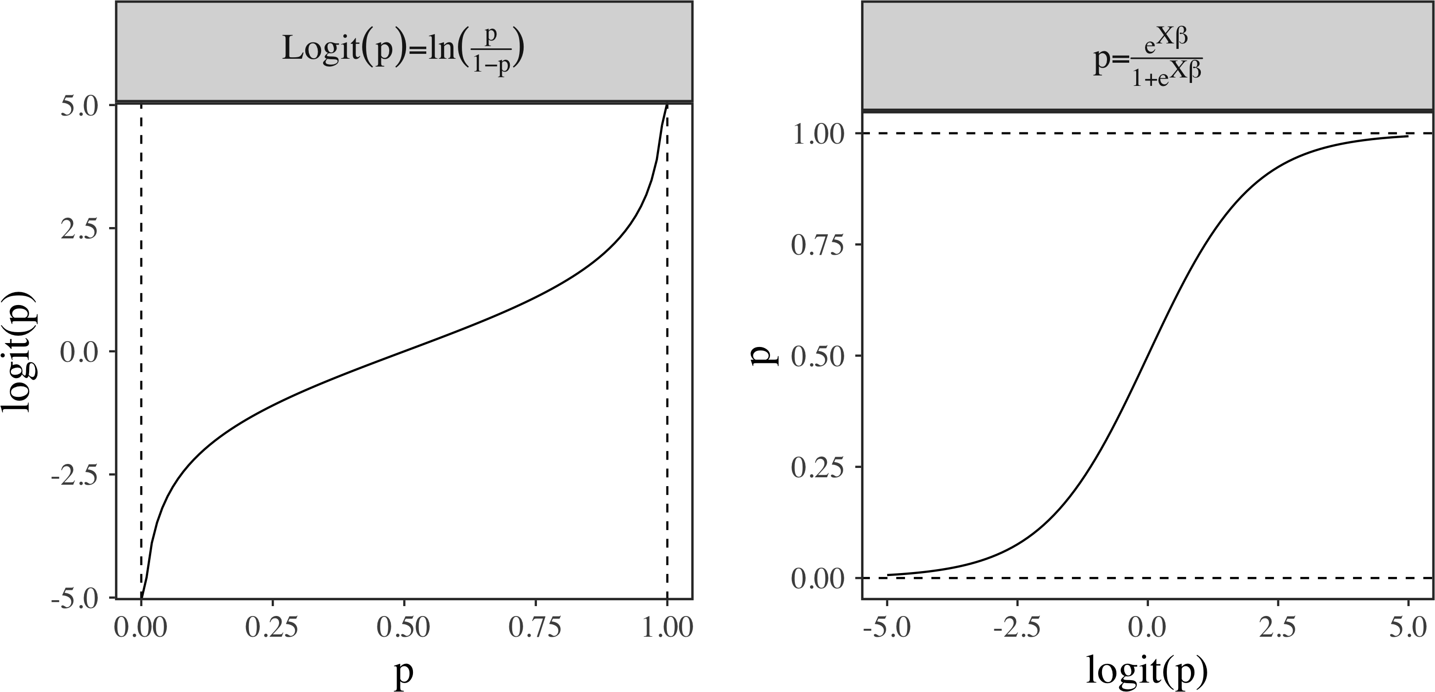
To better understand LR, we need to know logit and sigmoid functions and their relationship. The logit function or log-odds, $\text{logit}(p) = \log(\frac{p}{1-p})$, transforms a probability $p$ from $(0, 1)$ to the real range $(-\infty, \infty)$. By contrast, $\textrm{sigmoid}$ function, $\sigma(x) = \frac{e^x}{1 + e^x}$, converts a real value into a probability.
As you may expect, one function seems to be the inverse operation of the other. The truth is that the inverse of logit transformation is sigmoid function. We can proof this here.
\[\begin{split} y &= \log(\frac{x}{1-x}) \Rightarrow \text{switch probability of x and y in logit function} \\ x &= \log(\frac{y}{1-y}) \\ e^x &= \frac{y}{1-y} \\ e^x &= y + ye^x \\ y &= \frac{e^x}{1 + e^x} \Rightarrow \text{sigmoid function} \end{split}\]Now we can see that $\text{sigmoid}(x) = \text{logit}^{-1}(x)$. In stan manual, you may see $\text{logit}^{-1}(x)$ as an alternative for $\text{sigmoid}(x)$. Given a probability $p$, we will have $\sigma(\textrm{logit}(p)) = p$. Graphically, you can consider logit function as the mirror image of $\textrm{sigmoid}$ function along the line of $y = x$.

In the plot, $\text{logit}$ transform $p$ into real range and $\text{sigmoid}$ function inverses the transformation. Notice that I use the linear tranformation $X\beta$ in the $\text{sigmoid}$ function where $X$ is the design matrix and $\beta$ is the parameter vector (see next section for detailed explanation).
As a side note, you may know that there are some alternative terms for logit and sigmoid functions in the literature (see the table below). Here I will stick with logit/log-odds and sigmoid functions.
| $\text{logit}$ | $\text{sigmoid}$ |
|---|---|
| $\text{logit}$/log-odds | sigmoid/inverse logit/logistic |
3. Form
The formal representation of LR can be written below.
\[\begin{split} y &\sim Bernoulli(p) \\ p &= \frac{1}{1 + e^{-u}} \\ \mu &= X\beta \\ \beta_{k} &\sim \mathcal{N}(0, 10), ~ k = 1, ..., K \end{split}\]In this equation, the linear combinations of the design matrix $X$ and parameters $\beta$ will be first transformed via $\text{sigmoid}$ function to get the probability $p$, and further fed into the density of the Bernoulli distribution. Here I write the sigmoid function in another common way. You can get this new form by moving the numerator under the denominator. It is good to know that maximum likelihood estimation of Bernoulli distribution is equivalent to minimization of binary cross-entropy loss.
4. Data
We will first generate some random data points by using $p = \frac{exp(X\beta)}{1 + exp(X\beta)}$, which is equivalent to $\textrm{logit}(p) =X\beta$. Recall the relationship between sigmoid and logit functions, and try to proof this by yourself. Here we set $\beta = [-1, 1.2, 2.5]$ and $X \sim N(0, 1)$.
K <- 3 # intercept, x1 and x2
beta <- c(-1, 1.2, 2.5) # intercept and slope1 and slope2
N <- 500
# range of random X doesn't matter, here I am using centered data
X <- cbind(1, rnorm(N, 0, 1), rnorm(N, 0, 1))
linear_pred <- X %*% beta
prob <- exp(linear_pred) / (1 + exp(linear_pred)) # prob is a vector of probs
y <- rbinom(N, 1, prob)
5. Model
6. Run the analysis
MyData_logistic <- list(N = length(y), K = K, X = X, y = y)
fit_logistic <- sampling(stan_logit,
  data = MyData_logistic,
  chains = 1, iter = 2000, cores = 1, thin = 5,
)
7. Visualization
To visualize the predictive values of the fitted LR, I am using plotly package to draw the logistic regression surface below. In the interactive plot above, the yellow and purple points are the original data, and the red points indicate the fitted values on the surface. To better undertsand the marginal effects, I also fix $x_1$ and $x_2$ at certain values to show their marginal relationships with $y$, indicated by the red and blue lines in the plot.
Useful links:

