
Understanding Jacobian Adjustments for Constrained Parameters in Stan
Published:
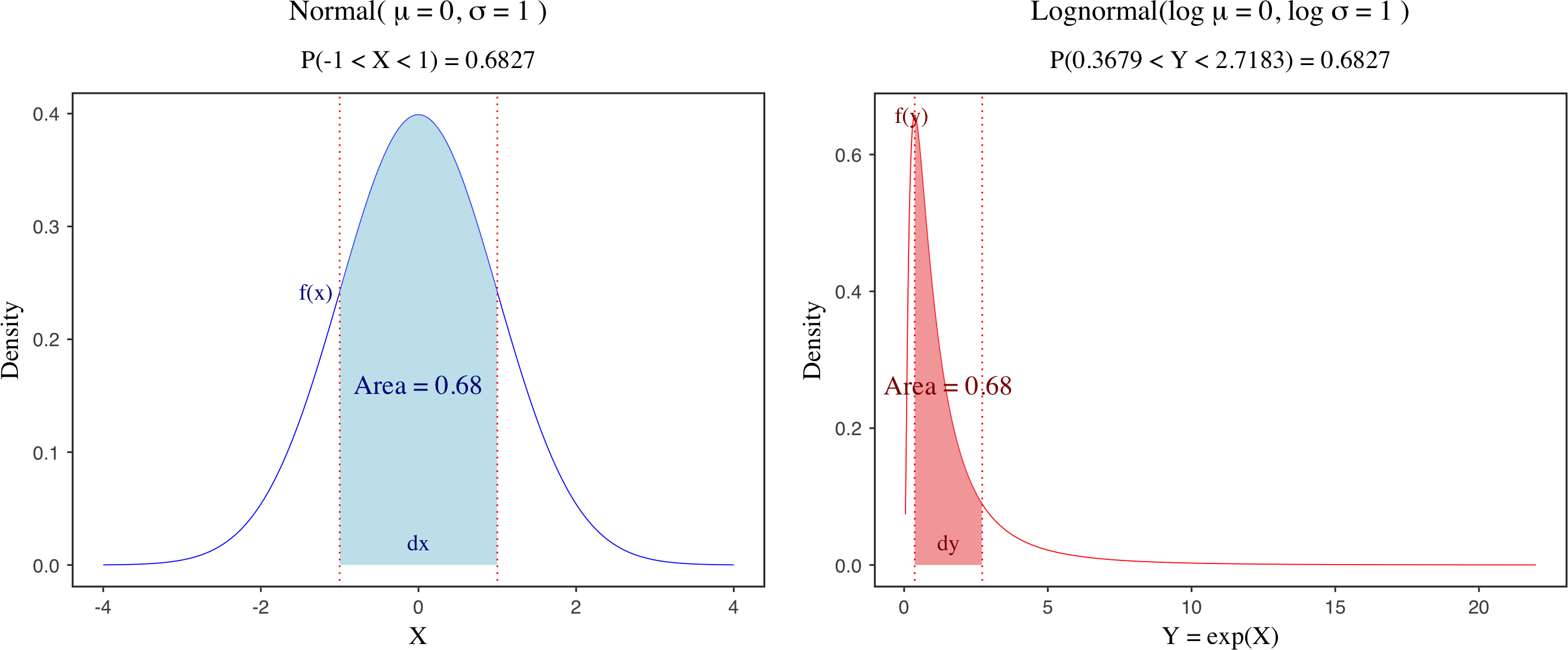
The Jacobian adjustment is a key concept in statistical modeling that arises when transforming probability distributions from one space to another. The intuition is that when you change a random variable, you’re not just changing the values - you’re also changing how “stretched” or “compressed” the probability density becomes at different points. To account for the distortion caused by the transform, the density must be multiplied by a Jacobian adjustment. This ensures that probability masses of corresponding intervals stay unchanged before and after the transform. This is illustrated by the figure above, which compares the probability density functions of a standard normal distribution and its transformed lognormal distribution. Although the shapes of the two distributions differ, the transformation must preserve the probability mass over corresponding intervals.
In Bayesian inference, Jacobian adjustments are especially important when transforming parameters from a constrained space (e.g., the positive real line) to an unconstrained space (e.g., the entire real line), which is commonly done to improve sampling efficiency and numerical stability. In Stan, such transformations are typically handled automatically. When you declare a constrained parameter (e.g., <lower=0>), Stan internally transforms it to an unconstrained space and applies the appropriate Jacobian adjustment to maintain the correct posterior density.
\[\left|f_Y(y) \cdot dy \right| = \left|f_X(x) \cdot dx \right|\]However, if you manually transform variables inside the transformed parameters block and assign priors to the transformed variables, you need to explicitly include the Jacobian adjustment to preserve the correct log posterior density (lp__). Failing to do so can lead to biased inference. To illustrate how this works, I’ll use a simple example of normal distribution, focusing on how Stan handles transformations of the standard deviation parameter $\sigma$ (i.e., <lower=0>) and how we can include a manual Jacobian adjustment.
1. Simulate data
I will first simulate some data from a normal distribution with mean 0 and standard deviation 20. A large standard deviation is chosen to make the effect of Jacobian adjustment more pronounced.
data_norm <- list(N = 100, y = rnorm(100, 0, 20))
2. Posterior parameter estimates
I will include three models to compare posterior parameter estimates and the log posterior density (lp__).
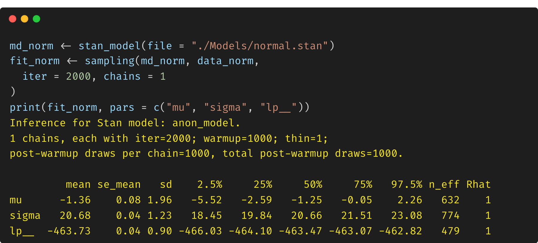
(1) Model 1: constrained parameter $\sigma$
The first model is a simple normal distribution with a proper constraint on $\sigma$ (<lower=0>). According to Stan reference manual, to avoid having to deal with constraints while simulating the Hamiltonian dynamics during sampling, every (multivariate) parameter in a Stan model is transformed to an unconstrained variable behind the scenes by the model compiler, and Stan handles the Jacobian adjustment automatically.
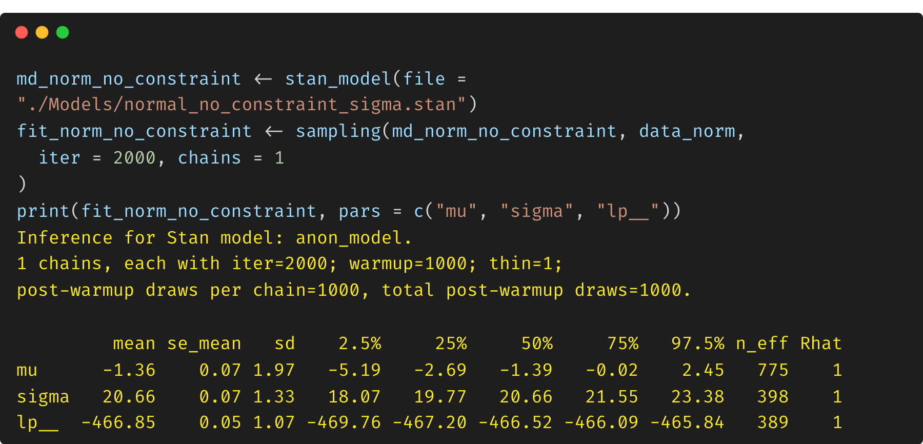
(2) Model 2: unconstrained parameter $\sigma$
Now we turn to another model by removing the constraint on $\sigma$. In this case, the parameter $\sigma$ is not a constrained variable, and there is no Jacobian adjustment handled by Stan. This means that the log posterior density (lp__) is biased.
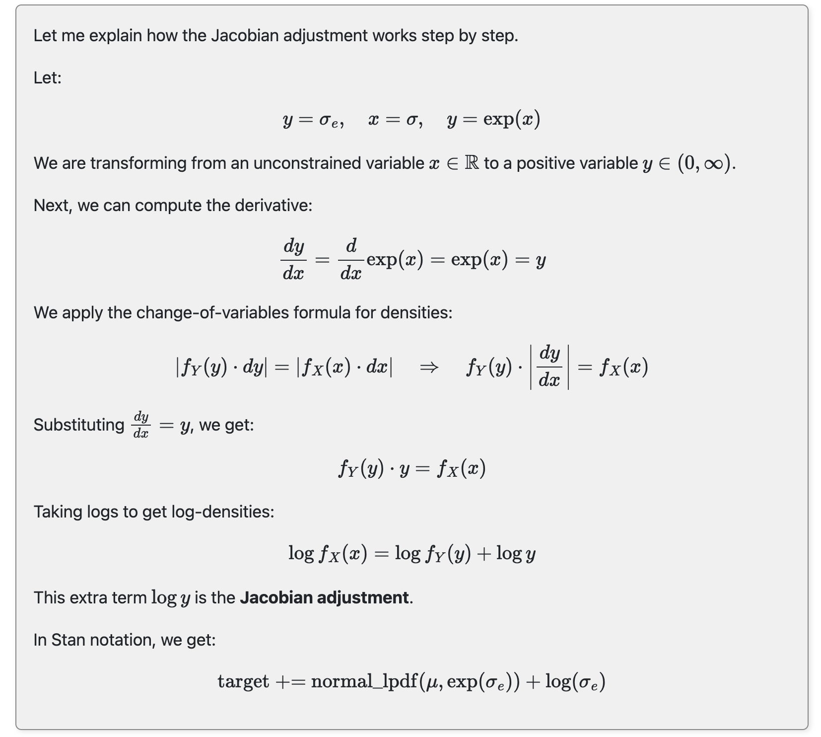
(3) Model 3: exponential transformation of unconstrained $\sigma$ and Jacobian adjustment
As a comparison, we can also reformulate the model by defining the parameter $\sigma$ as an unconstrained variable, and we then transform it via an exponential function (positive real line). The transformed variable $\sigma_{exp}$ will be assigned with a prior and used in the model. This is exactly what has happened internally by Stan when you define a parameter with a proper constraint (e.g., <lower=0>). Stan handles the transformation from an unconstrained internal representation to this constrained user-facing value. Thus, we need to include a Jacobian adjustment to preserve the correct log posterior density (lp__).
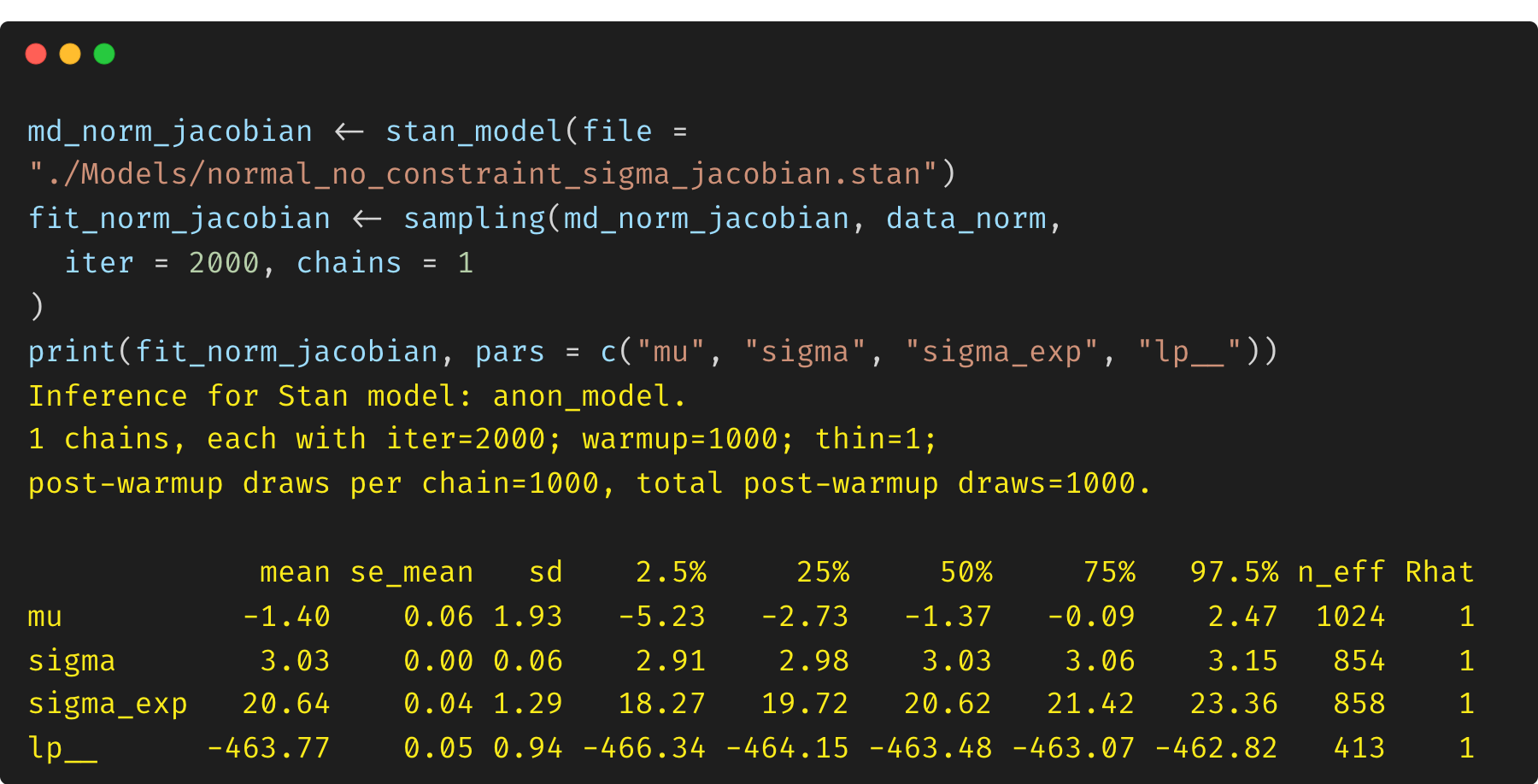
3. Comparison of results
As we can see, the posterior parameter estimates for $\mu$ and $\sigma$ are similar across all three models. However, the log posterior density (lp__) differs between Model 1 and Model 2. This is because Model 1 includes the proper constraint on $\sigma$, while Model 2 does not. The log posterior density in Model 2 is biased due to the missing Jacobian adjustment. Model 3 addresses this issue by including a Jacobian adjustment. In general, if you are interested in parameter inference, it may be not a major concern in this case, but missing Jacobian adjustments can cause serious problems for model comparison (e.g., WAIC, LOO, and Bayes factors).
Note that this example is only for illustration and help you understand the concept of Jacobian adjustment and how Stan handles changes of variables. In practice, you should always use the proper constraint on the parameter and let Stan handle the Jacobian adjustment automatically, which is both more efficient and more reliable.
Useful links
)](https://raw.githubusercontent.com/JakeJing/jakejing.github.io/master/_posts/pics/multi-logistic-reg-surface.png)