Multivariate Normal distribution and Cholesky decomposition in Stan
Published:
This post provides an example of simulating data in a Multivariate Normal distribution with given parameters, and estimating the parameters based on the simulated data via Cholesky decomposition in stan. Multivariate Normal distribution is a commonly used distribution in various regression models that generalize the Normal distribution into multidimensional space. Its PDF can be expressed as:
\(\text{MultiNormal}(y|\mu,\Sigma) = \frac{1}{\left( 2 \pi \right)^{k/2}} \ \frac{1}{\sqrt{|\Sigma|}} \ \exp \! \left( \! - \frac{1}{2} (y - \mu)^{\top} \, \Sigma^{-1} \, (y - \mu) \right) \!\) where $\mu$ is a vector of $k$ elements for the location and $\Sigma$ is the Variance-Covariance matrix. The $|\Sigma|$ calculates the absolute determinant of $\Sigma$ in the equation above.
Cholesky decomposition is used to decompose a positive-definite matrix into the product of a lower triangular matrix and its transpose. In our case, we will decompose the correlation matrix ($R$) into the product of two triangular matrices ($L_{u}*L_u^T$). Note: even though we can directly perform cholesky decomposition on the Variance-Covariance matrix ($\Sigma$), it is not recommended, since we may fail to estimate the standard deviations ($\sigma$) of each variable.
\[\begin{align*} \Sigma &= \left(\begin{array}{c}\sigma_{1}^2 ~~~~~~ \rho_{12}\sigma_{1}\sigma_{2} ~~~~~~ \rho_{13}\sigma_1\sigma_{3} \\ \rho_{12}\sigma_{1}\sigma_{2} ~~~~~~ \sigma_2^2 ~~~~~~ \rho_{23}\sigma_2\sigma_3 \\ \rho_{13}\sigma_1\sigma_{3} ~~~~~~ \rho_{23}\sigma_2\sigma_{3} ~~~~~~ \sigma_3^2 \end{array}\right)\\ \\ &= \left(\begin{array}{c}\sigma_1 ~~ 0 ~~ 0 \\ 0 ~~ \sigma_2 ~~ 0 \\ 0 ~~ 0 ~~ \sigma_3 \end{array}\right) \underbrace{\left(\begin{array}{c}1 ~~~ \rho_{12} ~~~ \rho_{13} \\ \rho_{12} ~~~ 1 ~~~ \rho_{23} \\ \rho_{13} ~~~ \rho_{23} ~~~ 1 \end{array}\right)}_{R} \left(\begin{array}{c}\sigma_1 ~~ 0 ~~ 0 \\ 0 ~~ \sigma_2 ~~ 0 \\ 0 ~~ 0 ~~ \sigma_3 \end{array}\right) \\ &= \left(\begin{array}{c} \sigma_1 ~~ 0 ~~ 0 \\ 0 ~~ \sigma_2 ~~ 0 \\ 0 ~~ 0 ~~ \sigma_3 \end{array}\right) \underbrace{L_uL_u^T}_{R} \left(\begin{array}{c} \sigma_1 ~~ 0 ~~ 0 \\ 0 ~~ \sigma_2 ~~ 0 \\ 0 ~~ 0 ~~ \sigma_3 \end{array}\right) \end{align*}\]1. Data simulation
The variance-covariance matrix ($\Sigma$) for data simulation and its analytical solution via Cholesky decomposition are provided below. For example, the standard deviation for the first variable $sd_1$ is $0.5$, and the correlation coefficient ($\rho$) between first and second variables is $0.7$.
\[\begin{align*} \Sigma &= \begin{pmatrix} 0.25 & 0.42 & 0.23\\ 0.42 & 1.44 & -1.38\\ 0.23 & -1.38 & 5.29 \end{pmatrix} \\ &= \begin{pmatrix} 0.5 & 0 & 0\\ 0 & 1.2 & 0\\ 0 & 0 & 2.3 \end{pmatrix} \times \underbrace{ \begin{pmatrix} 1 & 0.7 & 0.2 \\ 0.7 & 1 & -0.5 \\ 0.2& -0.5& 1 \end{pmatrix} }_{R} \times \begin{pmatrix} 0.5 & 0 & 0\\ 0 & 1.2 & 0\\ 0 & 0 & 2.3 \end{pmatrix} \\ &= \begin{pmatrix} 0.5 & 0 & 0\\ 0 & 1.2 & 0\\ 0 & 0 & 2.3 \end{pmatrix} \times \underbrace{\begin{pmatrix} 1 & 0 & 0 \\ 0.7 & 0.714 & 0 \\ 0.2& -0.896& 0.396 \\ \end{pmatrix}}_{L_{u}} \times \underbrace{ \begin{pmatrix} 1 & 0.7 & 0.2 \\ 0 & 0.714 & -0.896 \\ 0 & 0 & 0.396 \\ \end{pmatrix}}_{L_{u}^T} \times \begin{pmatrix} 0.5 & 0 & 0\\ 0 & 1.2 & 0\\ 0 & 0 & 2.3 \end{pmatrix} \end{align*}\]To generate the data, we are using the mvrnorm function from the package MASS.
mu = c(1, 2, -5) # means
R = matrix(c(1, 0.7, 0.2, # correlation matrix (R)
             0.7, 1, -0.5,
             0.2, -0.5, 1), 3)
sigmas = c(0.5, 1.2, 2.3) # sd1=0.5, sd2=1.2, sd3=2.3
Sigma = diag(sigmas) %*% R %*% diag(sigmas) # Variance-Covariance matrix
data = mvrnorm(1000, mu = mu, Sigma = Sigma) # data simulation
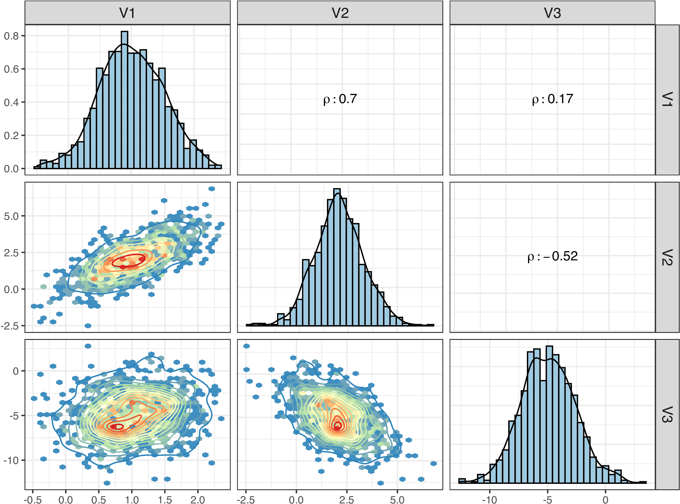
We plot the simulated data points as a pariwised contour plot, where the lower triangular panels show the mutual correlations and the upper triangular panels display the correlation coefficients ($\rho$).
2. Parameter estimation in stan
Here we are using a probabilistic programming language, stan, to estimate the parameters of the multivariate normal distribution based on the previously simulated data. The stan code block is attached below, and you can directly embed this chunk in R.
data {
  int<lower=1> N; // number of observations
  int<lower=1> K; // dimension of observations
  vector[K] y[N]; // observations: a list of K vectors
}
parameters {
  vector[K] mu;
  cholesky_factor_corr[K] Lcorr; // cholesky factor (L_u matrix for R)
  vector<lower=0>[K] sigma;
}
transformed parameters{
  corr_matrix[K] R; // correlation matrix
  cov_matrix[K] Sigma; // VCV matrix
  R = multiply_lower_tri_self_transpose(Lcorr);
  Sigma = quad_form_diag(R, sigma); // quad_form_diag: diag_matrix(sig) * R * diag_matrix(sig)
}
model {
  sigma ~ cauchy(0, 5); // prior for sigma
  Lcorr ~ lkj_corr_cholesky(2.0); // prior for cholesky factor
  y ~ multi_normal(mu, Sigma);
}
With the compiled stan model, we can start the sampling process and estimate the parameters.
input = list(N = 1000, K = 3, y = convertRowsToList(data))
results = sampling(stan_MVnorm_model, data=input,
                   chains = 4, iter = 2000, cores = 4)
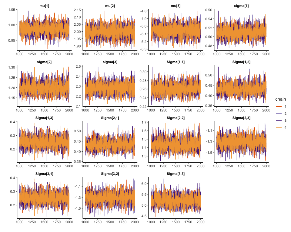
# mu[1]         0.99
# mu[2]         2.00
# mu[3]        -5.05
# sigma[1]      0.51
# sigma[2]      1.20
# sigma[3]      2.28
# Sigma[1,1]    0.26
# Sigma[1,2]    0.43
# Sigma[1,3]    0.25
# Sigma[2,1]    0.43
# Sigma[2,2]    1.44
# Sigma[2,3]   -1.31
# Sigma[3,1]    0.25
# Sigma[3,2]   -1.31
# Sigma[3,3]    5.20